Differential Geometry
Manifolds
Scalars, Vectors, Tensors
Differentiable manifold  is a space covered by an atlas of maps, each map
covers part of the manifold and is a one to one mapping to an euclidean space
is a space covered by an atlas of maps, each map
covers part of the manifold and is a one to one mapping to an euclidean space
 :
:

Let’s have a one-to-one transformation between  and
and  coordinates
(we simply write
coordinates
(we simply write  , etc.):


Scalar  is such a field that transforms as (
 is it’s value
in
is it’s value
in  coordinates):
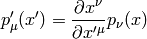
One form  is such a field that transforms the same as the
gradient
is such a field that transforms the same as the
gradient  of a scalar, that transforms as
(
of a scalar, that transforms as
( is it’s value in coordinates):
so
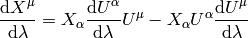
Vector  is such a field that produces a scalar
  when contracted with a one form and this fact is used to deduce how it
transforms:
when contracted with a one form and this fact is used to deduce how it
transforms:
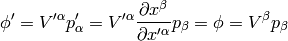
so we have
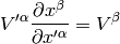
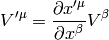
multiplying by  and using the fact that
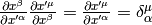 we get
Higher tensors are build up and their transformation properties derived from the fact, that by contracting with either a vector or a form we get a lower rank tensor that we already know how it transforms.
Having now defined scalar, vector and tensor fields, one may then choose a
basis at each point for each field, the only requirement being that the basis
is not singular. For example for vectors, each point in has a basis  , so a vector (field)
 has components with respect to this basis:

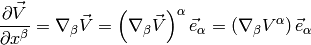
Covariant differentiation
The derivative of the basis vector  is a vector, thus it can be written as a linear
combination of the basis vectors:
is a vector, thus it can be written as a linear
combination of the basis vectors:

Differentiating a vector is then easy:

So we define a covariant derivative:
and write
I.e. we have:

We also define:

A scalar doesn’t depend on basis vectors, so its covariant derivative is just its partial derivative

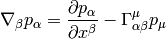
Differentiating a one form  is done using the fact, that
 is a scalar, thus

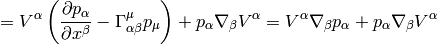
where we have defined
This is obviously a tensor, because the above equation has a tensor on the left
hand side ( ) and tensors on the right hand side
(
) and tensors on the right hand side
( and ). Similarly for the derivative of
the tensor
and ). Similarly for the derivative of
the tensor  we use the fact that
  is a
vector:
is a
vector:


where we define

and so on for other tensors, for example:


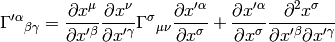
One can now easily proof some common relations simply by rewriting it to components and back:
Change of variable:
Parallel transport
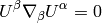
If the vectors at infinitesimally close points of the curve
 are parallel and of equal length, then is said to be
parallel transported along the curve, i.e.:
are parallel and of equal length, then is said to be
parallel transported along the curve, i.e.:

So
In components (using the tangent vector  ):
):
Fermi-Walker transport
In local inertial frame:

We require orthogonality  ,
in a general frame:
,
in a general frame:
where  was calculated by differentiating the orthogonality condition.
This is called a Thomas precession.
was calculated by differentiating the orthogonality condition.
This is called a Thomas precession.
For any vector, we define:
the vector  is Fermi-Walker tranported along the curve if:
If is perpendicular to  , the second term is zero and the result
is called a Fermi transport.
, the second term is zero and the result
is called a Fermi transport.
Why: the is transported by Fermi-Walker and also this is the equation
for gyroscopes, so the natural, nonrotating tetrade is the one with  , which is then correctly transported along any curve (not just
geodesics).
, which is then correctly transported along any curve (not just
geodesics).
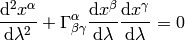
Geodesics
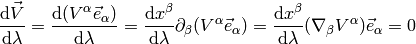
Geodesics is a curve  that locally looks like a line,
i.e. it parallel
transports its own tangent vector:
that locally looks like a line,
i.e. it parallel
transports its own tangent vector:
so
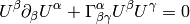
or equivalently (using the fact  ):
):
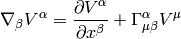
Curvature
Curvature means that we take a vector  , parallel transport it around
a closed loop (which is just applying a commutator of the covariant derivatives
, parallel transport it around
a closed loop (which is just applying a commutator of the covariant derivatives ![[\nabla_\alpha, \nabla_\beta]V^\mu](../../_images/math/4025c4f43eb0f72b83dd1890bfedaf45a492a82c.png) ), see how it changes and
that’s the curvature:
), see how it changes and
that’s the curvature:
![[\nabla_\alpha, \nabla_\beta]V^\mu\equiv R^\mu{}_{\nu\alpha\beta}V^\nu](../../_images/math/d2cdef901515168d83df026f3444947aaef21208.png)
That’s all there is to it. Expanding the left hand side:
![[\nabla_\alpha, \nabla_\beta]V^\mu=\left(\partial_\alpha\Gamma^\mu_{\beta\nu} -\partial_\beta\Gamma^\mu_{\alpha\nu} +\Gamma^\mu_{\alpha\sigma}\Gamma^\sigma_{\beta\nu} -\Gamma^\mu_{\beta\sigma}\Gamma^\sigma_{\alpha\nu}\right)V^\nu](../../_images/math/9469c66955886e1a1f84684ef37bd8c59dd24333.png)
we get

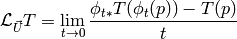
Lie derivative
Definition of the Lie derivative of any tensor  is:
is:
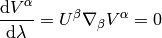
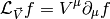
it can be shown directly from this definition, that the Lie derivative of a vector is the same as a Lie bracket:
![\L_{\vec U}\vec V \equiv [\vec U, \vec V]](../../_images/math/5bb166db7604da5f5a3cd904e0513b4c997b64d8.png)
and in components
![\L_{\vec U} V^\alpha = [\vec U, \vec V]^\alpha\equiv U^\beta\nabla_\beta V^\alpha- V^\beta\nabla_\beta U^\alpha = U^\beta\partial_\beta V^\alpha- V^\beta\partial_\beta U^\alpha](../../_images/math/a004056d65888aedb6aaacd9ca6d08c7c3f2d1ab.png)
Lie derivative of a scalar is
and of a one form  is derived using the observation that
  is a scalar:

and so on for other tensors, for example:

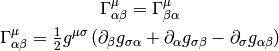
Metric
In general, the Christoffel symbols are not symmetric and there is no metric that generates them. However, if the manifold is equipped with metrics, then the fundamental theorem of Riemannian geometry states that there is a unique Levi-Civita connection, for which the metric tensor is preserved by parallel transport:

We define the commutation coefficients of the basis  by
by
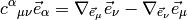
In general these coefficients are not zero (as an example, take the units vectors in spherical or cylindrical coordinates), but for coordinate bases they are. It can be proven, that

and for coordinate bases  , so
, so
As a special case:
All last 3 expressions are used (but the last one is probably the most common).
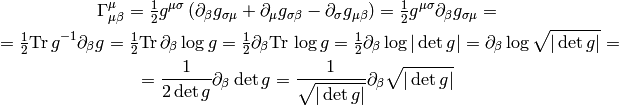
 is the matrix of coefficients
  . At the beginning we used the
usual trick that
. At the beginning we used the
usual trick that  is symmetric but
 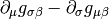 is unsymmetric. Later we used
the identity
is unsymmetric. Later we used
the identity 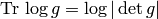 , which follows from the well-known
identity
, which follows from the well-known
identity  by substituting
  and taking the
logarithm of both sides.
and taking the
logarithm of both sides.
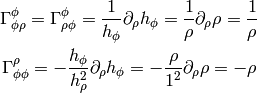
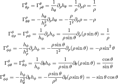
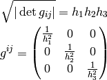
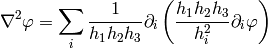
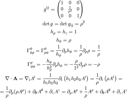
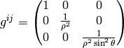
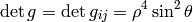
Diagonal Metric
Many times the metric is diagonal, e.g. in 3D:
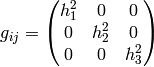
(in general 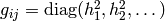 ), then the Christoffel
symbols
), then the Christoffel
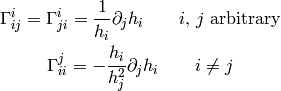
symbols  can be calculated very easily (below we do not sum
over
can be calculated very easily (below we do not sum
over  ,
,  and
and  ):
):

If  or
or  then
then
(1)
otherwise (i.e.  and
and  ) then either
  :
:
(2)
or  (i.e.
(i.e.  ):
):

In other words, the symbols can only be nonzero if at least two of ,
or are the same and one can use the two formulas (1) and
(2) to quickly evaluate them. A systematic way to do it is to write
(1) and (2) in the following form:
(3)
Then find all and for which  is nonzero and then
immediately write all nonzero Christoffel symbols using the equations
(3).
is nonzero and then
immediately write all nonzero Christoffel symbols using the equations
(3).
For example for cylindrical coordinates we have  and
and  , so is only nonzero for
  and
and  and we
get:
and we
get:
all other Christoffel symbols are zero. For spherical coordinates we have
 ,
,  and
and  , so is
only nonzero for
, so is
only nonzero for  , or , or ,
 and we get:
All other symbols are zero.
Symmetries, Killing vectors
We say that a diffeomorphism  is a symmetry of some tensor T if the
tensor is invariant after being pulled back under :
is a symmetry of some tensor T if the
tensor is invariant after being pulled back under :

Let the one-parameter family of symmetries  be generated by a vector
field
be generated by a vector
field  , then the above equation is equivalent to:

If is the metric then the symmetry is called isometry and
is called a Killing vector field and can be calculated from:

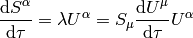
The last equality is Killing’s equation. If is a geodesics with a
tangent vector and is a Killing vector, then the quantity
 is conserved along the geodesics, because:

where the first term is both symmetric and antisymmetric in  , thus
zero, and the second term is the geodesics equation, thus also zero.
, thus
zero, and the second term is the geodesics equation, thus also zero.
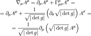
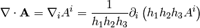
Covariant integration
If  is a scalar, then the integral
  depends on
coordinates. The correct way to integrate in any coordinates is:
depends on
coordinates. The correct way to integrate in any coordinates is:
where  . The Gauss theorem in curvilinear coordinates
is:
. The Gauss theorem in curvilinear coordinates
is:
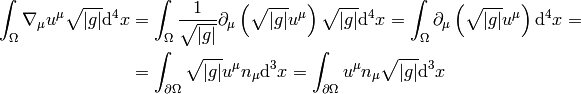
where  is the boundary (surface) of
  and
and  is the
normal vector to this surface.
is the
normal vector to this surface.
Examples
Weak Formulation of Laplace Equation
As an example, we write the weak formulation of the Laplace equation in arbitrary coordintes:
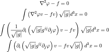
Now we apply per-partes (assuming the boundary integral vanishes):

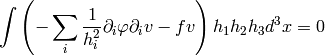
For diagonal metric this evaluates to:
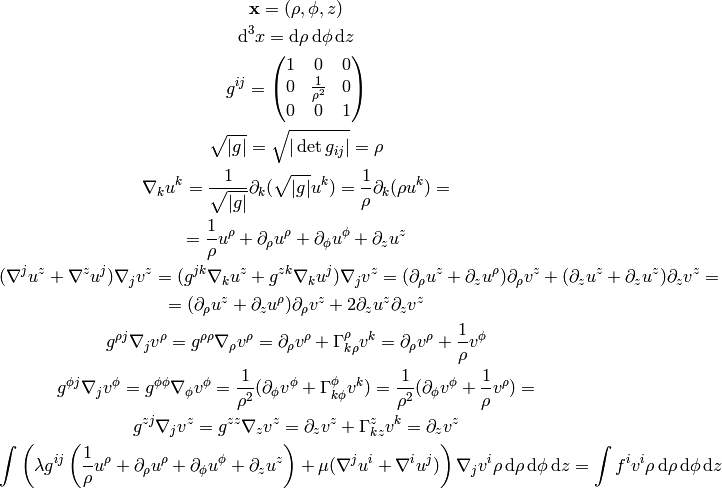
Cylindrical Coordinates


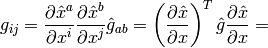
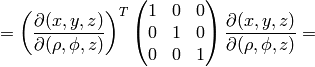
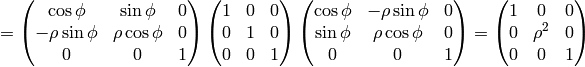
The transformation matrix is
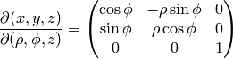
The metric tensor of the cartesian coordinate system 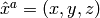 is
is
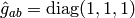 ,
so by transformation we get the metric tensor
,
so by transformation we get the metric tensor  in the cylindrical
coordinates
in the cylindrical
coordinates  :
:
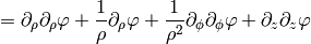
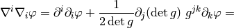
As a particular example, let’s write the Laplace equation with nonconstant conductivity for axially symmetric field. The Laplace equation is:

so we use the formulas above to get:

but we know that  , so
, so
 and the final equation is:
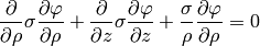
To write the weak formulation for it, we need to integrate covariantly (e.g.
 in our case) and
rewrite it using per partes. We did exactly this in the previous example in a
coordinate free maner, so we just use the final formula we got there for a
diagonal metric:
in our case) and
rewrite it using per partes. We did exactly this in the previous example in a
coordinate free maner, so we just use the final formula we got there for a
diagonal metric:
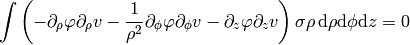
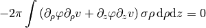
and for  , we get:
Spherical Coordinates

The transformation matrix is
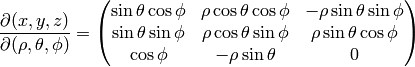
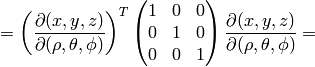
The metric tensor of the cartesian coordinate system is
,
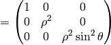
so by transformation we get the metric tensor in the spherical
coordinates  :
:


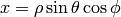
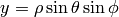
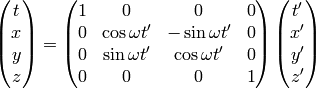
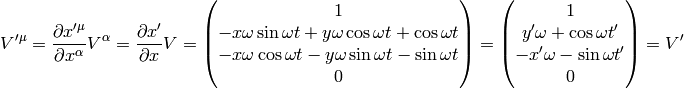
Rotating Disk
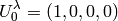
Let’s have a laboratory Euclidean system  and
a rotating disk system
and
a rotating disk system 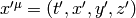 . The relation between the frames is
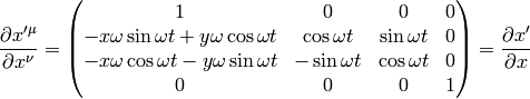
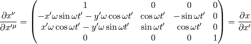
The inverse transformation can be calculated by simply inverting the matrix:
so the transformation matrices are:
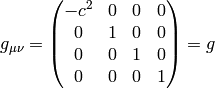
The problem now is that Newtonian mechanics has a degenerated spacetime
metrics (see later). Let’s pretend we have the following metrics in the
system:
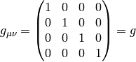
and
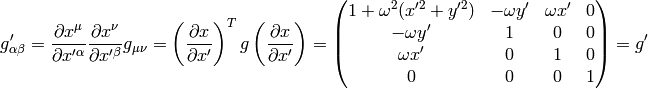
However, if we calculate with the correct special relativity metrics:
and
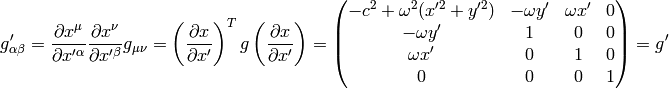
We get the same Christoffel symbols as with the  metrics,
because only the derivatives of the metrics are important.
Then the only nonzero Christoffel symbols are
metrics,
because only the derivatives of the metrics are important.
Then the only nonzero Christoffel symbols are


If we want to avoid dealing with metrics, it is possible
to
start with the Christoffel symbols in the system:

and then transforming them to the system using the change of variable
formula:

As an example, let’s calculate the coefficients above:
So we got the same results.
Now let’s see what we have got.
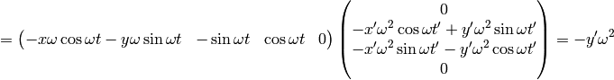
Later we’ll show, that the  coefficients are just
 in the Newtonian theory. E.g. in our case we have:
from which:

and the force acting on a test particle is then:

where we have defined  . This is just the centrifugal
force. Also observe, that we could have read directly from the metrics
itself — just compare it to the Lorentzian metrics (with gravitation) in the
next chapter.
. This is just the centrifugal
force. Also observe, that we could have read directly from the metrics
itself — just compare it to the Lorentzian metrics (with gravitation) in the
next chapter.
The other two terms ( ,
,  and the symmetric ones) don’t behave as a gravitational force, but
rather only act when we are differentiating (e.g. only act on moving bodies).
Below we show this is just the
and the symmetric ones) don’t behave as a gravitational force, but
rather only act when we are differentiating (e.g. only act on moving bodies).
Below we show this is just the  term
(responsible for the Coriolis acceleration).
term
(responsible for the Coriolis acceleration).
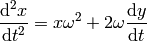
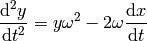
Let’s write the full equations of geodesics:

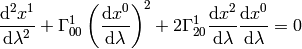
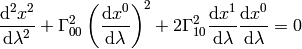

This becomes:

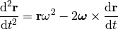
we can define  and
and  . Then the
above equations can be rewritten as:
. Then the
above equations can be rewritten as:
So we get two fictituous forces, the centrifugal force and the Coriolis force.
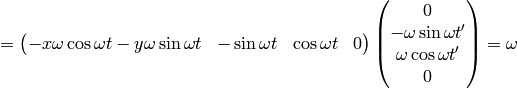
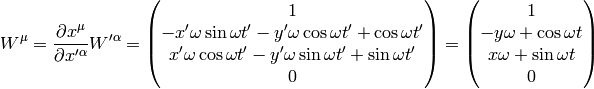
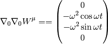
Now imagine a static vector in the system along the  axis, i.e.
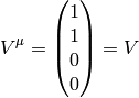
then
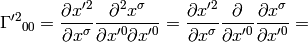
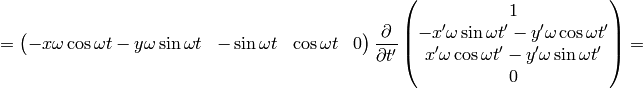
In the last equality we transformed from to using the
relation between frames.
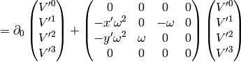
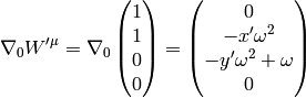
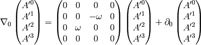
Differentiating any vector in the coordinates
is easy – it’s just a partial derivative (due to the Euclidean metrics).
Let’s differentiate any vector in the
coordinates with respect to time (since  , the time is the same in both
coordinate systems):
, the time is the same in both
coordinate systems):

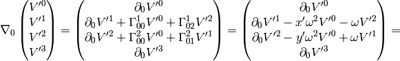
(4)
For our particular (static) vector this yields:
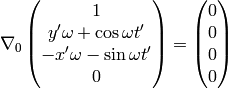
as expected, because it was at rest in the system.
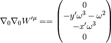
Let’s imagine a static vector in the system along the axis, i.e.

then
Similarly
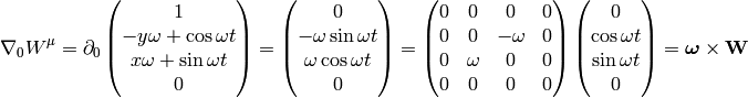
How can one prove the relation:
(5)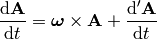
that is used for example to derive the Coriolis acceleration etc.? We need to write it components to understand what it really means:
Comparing to the covariant derivative above, it’s clear that they are equal
(provided that  and
and  , i.e. we are at the center of rotation).
Let’s show the derivation by Goldstein. The change in a time  of a
general vector
of a
general vector  as seen by an observer in the body system of axes will
differ from the corresponding change as seen by an observer in the space
system:
as seen by an observer in the body system of axes will
differ from the corresponding change as seen by an observer in the space
system:

Now consider a vector fixed in the rigid body. Then 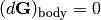 and
and

For an arbitrary vector, the change relative to the space axes is the sum of the two effects:

A more rigorous derivation of the last equation follows from:

Let’s make the space and body instantaneously coincident at time t, then
 and
and
 , so
we get the same equation as earlier:
, so
we get the same equation as earlier:
Anyhow, introducing  by:
by:

we get
Linear Elasticity Equations in Cylindrical Coordinates
Authors: Pavel Solin & Lenka Dubcova
In this paper we derive the weak formulation of linear elasticity equations suitable for the finite element discretization of axisymmetric 3D problems.
Original equations in Cartesian coordinates
Let’s start with some notations: By  we denote the displacement vector in
3D Cartesian coordinates, and by
we denote the displacement vector in
3D Cartesian coordinates, and by  the tensor of small deformations,
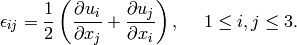
The stress tensor  has the form
(6)
where
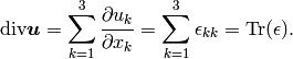
The symbols and  are the Lam’e constants and
  is the Kronecker
symbol (
is the Kronecker
symbol ( if
if  and
and  otherwise).
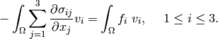
The equilibrium equations have the form
otherwise).
The equilibrium equations have the form
(7)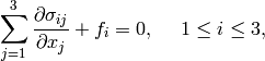
where  is the vector of internal forces (such as gravity).
The boundary conditions for linear elasticity are given by
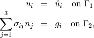
where  are surface forces.
Weak formulation
Multiplying by test functions and integrating over the domain we obtain
(8)
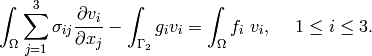
Using Green’s theorem and the boundary conditions
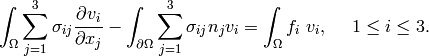
Thus
(9)
Let us write the equations (9) in detail using relation (6)
(10)![\begin{eqnarray*}
\int_{\Omega} \left[\lambda \mbox{div}u + 2 \mu \frac{\partial u_1}{\partial x_1}\right] \frac{\partial v_1}{\partial x_1} + \mu \left(\frac{\partial u_1}{\partial x_2} + \frac{\partial u_2}{\partial x_1}\right)\frac{\partial v_1}{\partial x_2} + \mu \left(\frac{\partial u_1}{\partial x_3} + \frac{\partial u_3}{\partial x_1}\right)\frac{\partial v_1}{\partial x_3}
- \int_{\Gamma_2} g_1 v_1 &=& \int_{\Omega}f_1\ v_1,\nonumber\\
\int_{\Omega} \mu \left(\frac{\partial u_1}{\partial x_2} + \frac{\partial u_2}{\partial x_1}\right)\frac{\partial v_2}{\partial x_1} + \left[\lambda \mbox{div}u + 2 \mu \frac{\partial u_2}{\partial x_2}\right] \frac{\partial v_2}{\partial x_2} + \mu \left(\frac{\partial u_2}{\partial x_3} + \frac{\partial u_3}{\partial x_2}\right)\frac{\partial v_2}{\partial x_3}
- \int_{\Gamma_2} g_2 v_2 &=& \int_{\Omega}f_2\ v_2,\\
\int_{\Omega} \mu \left(\frac{\partial u_1}{\partial x_3} + \frac{\partial u_3}{\partial x_1}\right)\frac{\partial v_3}{\partial x_1} + \mu \left(\frac{\partial u_2}{\partial x_3} + \frac{\partial u_3}{\partial x_2}\right)\frac{\partial v_3}{\partial x_2} + \left[\lambda \mbox{div}u + 2 \mu \frac{\partial u_3}{\partial x_3}\right] \frac{\partial v_3}{\partial x_3}
- \int_{\Gamma_2} g_3 v_3 &=& \int_{\Omega}f_3\ v_3.\nonumber
\end{eqnarray*}](../../_images/math/0b77882aca2c10d5218be959780c7dd18ef18d8c.png)
Elementary transformation relations
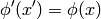
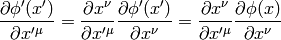
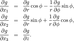
First let us show how the partial derivatives of a scalar function are transformed
from Cartesian coordinates  to cylindrical coordinates
  .
Note that
.
Note that

Since

it is
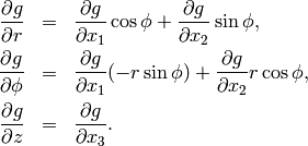
From here we obtain
(11)
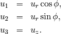
The relations between displacement components in Cartesian and cylindrical coordinates are
(12)
The same relations hold for surface forces and volume forces  .
.
Applying (11) to  , we obtain
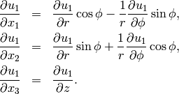
Using (12) and the fact that  does not depend on , this yields
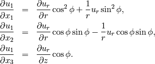
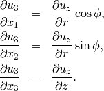
Analogously, for  we calculate
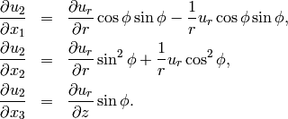
For  , using that it does not depend on , we have
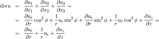
For further reference, transform also  into cylindrical
coordinates
into cylindrical
coordinates
Axisymmetric formulation
Assuming that the domain is axisymmetric,
we can begin to transform the integrals in (10) to cylindrical coordinates.
Recall that the Jacobian of the transformation is 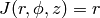 . The first equation in (10) has the form:
![\begin{eqnarray*} &&\int_{\Omega} r \left[\lambda (\frac{\partial u_r}{\partial r} + \frac{1}{r} u_r + \frac{\partial u_z}{\partial z}) + 2 \mu (\frac{\partial u_r}{\partial r}\cos^2\phi + \frac{1}{r} u_r\sin^2\phi)\right] (\frac{\partial v_r}{\partial r}\cos^2\phi + \frac{1}{r} v_r\sin^2\phi) + \\ &&r 2 \mu \left(\frac{\partial u_r}{\partial r}\cos\phi\sin\phi - \frac{1}{r}u_r \cos\phi\sin\phi\right)\left(\frac{\partial v_r}{\partial r}\cos\phi\sin\phi - \frac{1}{r}v_r \cos\phi\sin\phi\right) + \\ &&r \mu \left(\frac{\partial u_r}{\partial z}\cos\phi + \frac{\partial u_z}{\partial r}\cos\phi\right)\frac{\partial v_r}{\partial z}\cos\phi - \int_{\Gamma_2} r g_r v_r {\cos}^2 \phi = \int_{\Omega} r f_r\ v_r \cos^2 \phi, \end{eqnarray*}](../../_images/math/8f4c3c83c1f58a88675c241860d639c4ea5bacc7.png)
The second equation in (10) has the form:
![\begin{eqnarray*} &&\int_{\Omega} r 2\mu \left(\frac{\partial u_r}{\partial r}\cos\phi\sin\phi - \frac{1}{r}u_r \cos\phi\sin\phi\right)\left(\frac{\partial v_r}{\partial r}\cos\phi\sin\phi - \frac{1}{r}v_r \cos\phi\sin\phi\right) +\\ && r \left[\lambda (\frac{\partial u_r}{\partial r} + \frac{1}{r} u_r + \frac{\partial u_z}{\partial z}) + 2 \mu (\frac{\partial u_r}{\partial r}\sin^2\phi + \frac{1}{r} u_r\cos^2\phi)\right] (\frac{\partial v_r}{\partial r}\sin^2\phi + \frac{1}{r} v_r\cos^2\phi) + \\ && r \mu \left(\frac{\partial u_r}{\partial z}\sin\phi + \frac{\partial u_z}{\partial r}\sin\phi\right)(\frac{\partial v_r}{\partial z}\sin\phi) - \int_{\Gamma_2}r g_r v_r \sin^2 \phi = \int_{\Omega}r f_r\ v_r \sin^2 \phi,\\ \end{eqnarray*}](../../_images/math/429554da8cce51abf005b30717dcf453d97049eb.png)
Adding these two equations together we get
![\begin{eqnarray*} &&\int_{\Omega} r \lambda (\frac{\partial u_r}{\partial r} + \frac{1}{r} u_r + \frac{\partial u_z}{\partial z}) (\frac{\partial v_r}{\partial r} + \frac{1}{r} v_r) + \\ &&\int_{\Omega} r \mu \left[ 2 \left(\frac{\partial u_r}{\partial r}\frac{\partial v_r}{\partial r}\cos^4\phi + \frac{1}{r} u_r \frac{\partial v_r}{\partial r}\sin^2 \phi \cos^2 \phi + \frac{1}{r}\frac{\partial u_r}{\partial r} v_r\sin^2 \phi \cos^2 \phi + \frac{1}{r^2} u_r v_r\sin^4\phi\right) +\right.\\ &&\qquad\ \left.2 \left(\frac{\partial u_r}{\partial r}\frac{\partial v_r}{\partial r}\sin^4\phi + \frac{1}{r} u_r \frac{\partial v_r}{\partial r}\sin^2 \phi \cos^2 \phi + \frac{1}{r}\frac{\partial u_r}{\partial r} v_r\sin^2 \phi \cos^2 \phi + \frac{1}{r^2} u_r v_r\cos^4\phi\right) + \right. \\ && \left. 4 \left( \frac{\partial u_r}{\partial r}\frac{\partial v_r}{\partial r}\cos^2\phi\sin^2\phi - \frac{1}{r}u_r\frac{\partial v_r}{\partial r} \cos^2\phi\sin^2\phi - \frac{1}{r} \frac{\partial u_r}{\partial r} v_r \cos^2\phi\sin^2\phi + \frac{1}{r^2}u_r v_r \cos^2\phi\sin^2\phi\right)\right. + \\ && \left. \left(\frac{\partial u_r}{\partial z}\frac{\partial v_r}{\partial z} + \frac{\partial u_z}{\partial r}\frac{\partial v_r}{\partial z}\right)\right] - \int_{\Gamma_2} g_r v_r r= \int_{\Omega}f_r\ v_r r \end{eqnarray*}](../../_images/math/891bfd06b0634a09706c062f4db3e61b77b6f7af.png)
This can be simplified to
![\int_{\Omega} r \lambda (\frac{\partial u_r}{\partial r} + \frac{1}{r} u_r + \frac{\partial u_z}{\partial z}) (\frac{\partial v_r}{\partial r} + \frac{1}{r} v_r) + \int_{\Omega} r \mu \left[ 2 \left(\frac{\partial u_r}{\partial r}\frac{\partial v_r}{\partial r} + \frac{1}{r^2} u_r v_r\right) + \left(\frac{\partial u_r}{\partial z}\frac{\partial v_r}{\partial z} + \frac{\partial u_z}{\partial r}\frac{\partial v_r}{\partial z}\right)\right]](../../_images/math/01684fd99a3744058a7cf3695e197adb71350704.png)
Finally, the third equation in (10) has the form
![\begin{eqnarray*} && \int_{\Omega} r \mu \left(\frac{\partial u_r}{\partial z}\cos\phi + \frac{\partial u_z}{\partial r}\cos\phi\right)\frac{\partial v_z}{\partial r}\cos\phi + r \mu \left(\frac{\partial u_r}{\partial z}\sin\phi + \frac{\partial u_z}{\partial r}\sin\phi\right)\frac{\partial v_z}{\partial r}\sin\phi + \\ && r \left[\lambda (\frac{\partial u_r}{\partial r} + \frac{1}{r} u_r + \frac{\partial u_z}{\partial z} ) + 2 \mu \frac{\partial u_z}{\partial z}\right] \frac{\partial v_z}{\partial z} - \int_{\Gamma_2} g_z v_z r = \int_{\Omega}f_z\ v_z r. \end{eqnarray*}](../../_images/math/2dfe4705fb5a690fc4ad1699b8d852df0b4bc777.png)
This gives us

Since the integrands do not depend on , we can simplify this to integral over  , where is the intersection of the domain with the
  half-plane. Dividing both equations by
  we get
![\int_{\Omega_0} r \lambda (\frac{\partial u_r}{\partial r} + \frac{1}{r} u_r + \frac{\partial u_z}{\partial z}) (\frac{\partial v_r}{\partial r} + \frac{1}{r} v_r) + \int_{\Omega_0} r \mu \left[ 2 \left(\frac{\partial u_r}{\partial r}\frac{\partial v_r}{\partial r} + \frac{1}{r^2} u_r v_r\right) + \left(\frac{\partial u_r}{\partial z}\frac{\partial v_r}{\partial z} + \frac{\partial u_z}{\partial r}\frac{\partial v_r}{\partial z}\right)\right]](../../_images/math/5e4ed98ecf69a49035ce00187f1c14e3c300a933.png)

Coordinate Independent Way
Let’s write the elasticity equations in the cartesian coordinates again:
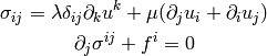
Those only work in the cartesian coordinates, so we first write them in a coordinate independent way:
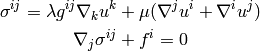
so:

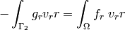
The weak formulation is then (do not sum over ):

We apply the integration by parts:

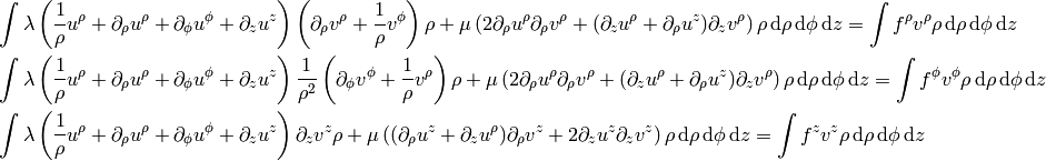
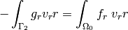
This is the weak formulation valid in any coordinates. Using the cylindrical coordinates (see above) we get:
for  we get: